Good Modeling Practices - Matrix Notation
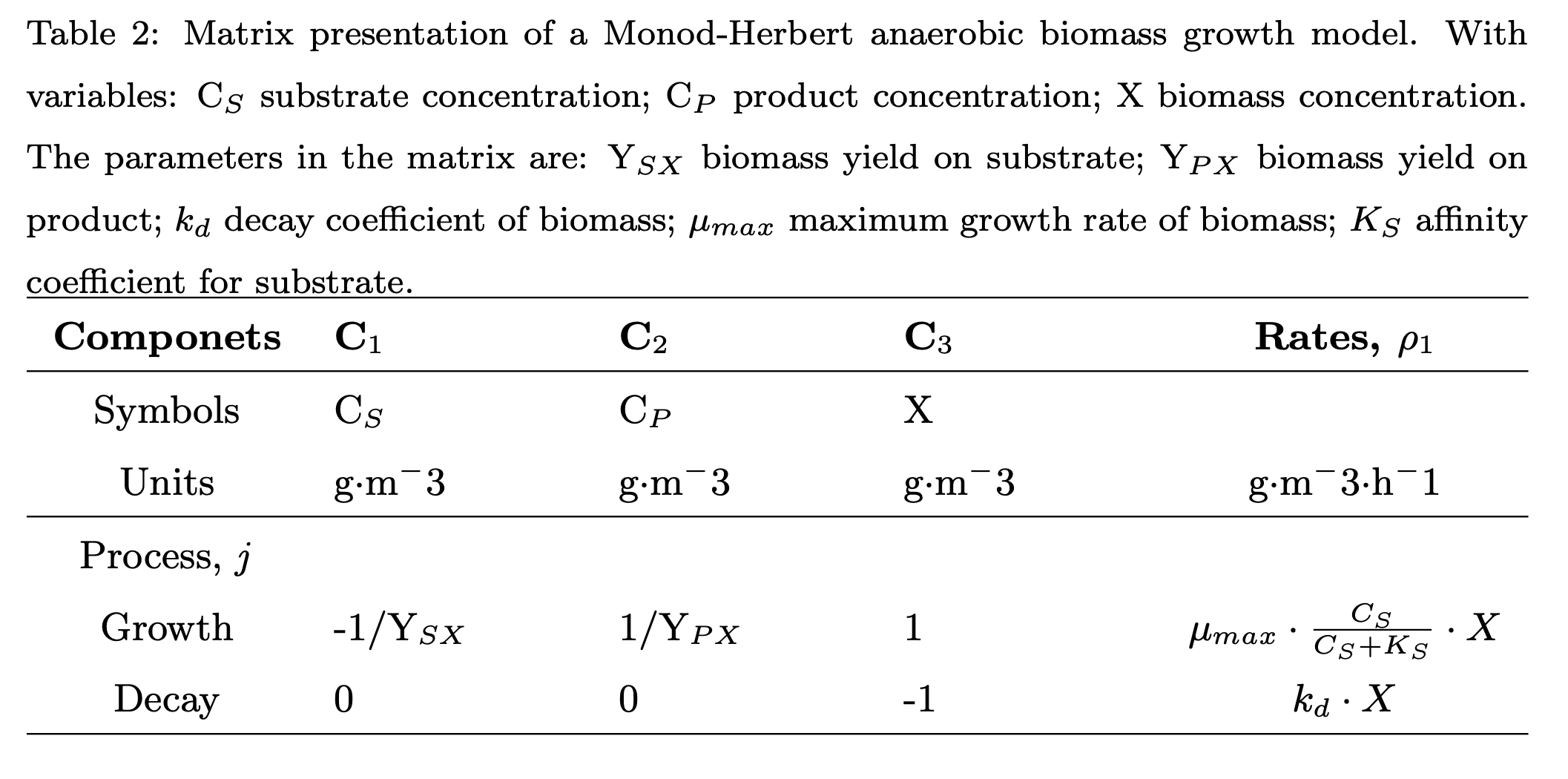
Matrix notation uses the linear relations among net conversion rates in order to describe the conservation relations inside a system and it is is a well established system to mathematically describe complex models. The description of a system through this methodology is done by defining its number of components n, and its number of processes m. This is the foundation for the stoichiometric matrix, S, the process rate vector, ρ, and finally, the component conversion rate vector r.
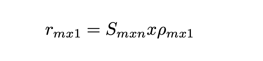
The overall component conversion rate vector (r) is then coupled to a general mass balance equation.
Template example
from scipy.integrate import odeint
import math
import numpy as np

class name_of_your_model:
    def __init__(self):
        #Fill up with your parameters
        #Example: self.Y_XS = 0.8 #g/g

        #Initialization of state variable
        #Example: self.S0 = 18

    def rxn(self, C, t):
        #number of components (n = )
        #number of processes (m = )

        #initialize the stoichiometric matrix (e.g. s)
        #s = np.zeros((m,n))

        #We define each value of the matrix
        #Example: self.s[0,0]=(-1/self.Y_XS)

        #initialize the process vector (e.g. rho)
        #rho = np.zeros((m,1))

        #We define each value of the process rate vector
        ##Example: rho[0,0] = self.mu_max*(C[0]/(C[0]+self.Ks))*C[2]

        #the overall conversion rate is stoichiometric *rates
        ##Example: self.r[0,0]= self.s[0,0]*self.rho[0,0]+self.s[1,0]*self.rho[1,0]+(s[2,0]*rho[2,0])

        #Then, it is solved the mass balances, in this case discontinuous:
        ##Example: dSdt = self.r[0,0]
        return [dSdt,...]

    def solve(self):
        #Create a vector that shows the initial time to solve the model
        #t = np.linspace(t0, tf)

        #Vector with the initial conditions of the state variables
        #C0 = [self.S0,.....]

        #The ODE solver
        #C = odeint(self.rxn, C0, t, rtol = 1e-7, mxstep= 500000)
        return t, C

#How to call the model so it is printed.
t, C = Model().solve()
Example
A (bio)kinetic first-principle model. In this case, for the representation of the aerobic growth of textit{Corynebacterium glutamicum} under product inhibition.
# -*- coding: utf-8 -*-
"""
Created on Wed Jan 23 10:42:13 2019

@author: simoca
"""

from scipy.integrate import odeint
#Package for plotting
import math
#Package for the use of vectors and matrix
import numpy as np
import pandas as pd
import array as arr
from matplotlib.backends.backend_qt5agg import FigureCanvasQTAgg as FigureCanvas
from matplotlib.figure import Figure
import sys
import os
import matplotlib.pyplot as plt
from matplotlib.ticker import FormatStrFormatter
import glob
from random import sample
import random
import time
import plotly
import plotly.graph_objs as go
import json
from plotly.subplots import make_subplots


class CGlutamicum_aerobic:
    def __init__(self, Control = False):
        self.mu_max= 0.21 #h^-1
        self.Kg=0.8 #g/L
        self.nu=1
        self.Yxs=0.149#g/g
        self.Ypx=3.278 #g/g
        self.Yps=0.48 #g/g
        self.Pcritical=11.529#g/L
        self.kd=0.1


        #Initial concentrations
        self.X0= 0.164 #g/L
        self.P0=0.2#g/L
        self.S0=49.87 #g glucose/L
        self.V0= 2 #L

        self.t_end=30
        self.t_start=0

        #parameters for control, default every 1/24 hours:
        self.Control = Control
        self.coolingOn = True
        self.Contamination=False
        self.steps = (self.t_end - self.t_start)*24
        self.T0 = 30
        self.K_p = 2.31e+01
        self.K_i = 3.03e-01
        self.K_d = -3.58e-03
        self.Tset = 30
        self.u_max = 150
        self.u_min = 0

    def rxn(self, C,t , u, fc):
        if self.Control == True :
            #Cardinal temperature model with inflection: Salvado et al 2011 "Temperature Adaptation Markedly Determines Evolution within the Genus Saccharomyces"
            #Strain S. cerevisiae PE35 M
            Topt = 30
            Tmax = 45.48
            Tmin = 5.04
            T = C[5]
            if T < Tmin or T > Tmax:
                 k = 0
            else:
                 D = (T-Tmax)*(T-Tmin)**2
                 E = (Topt-Tmin)*((Topt-Tmin)*(T-Topt)-(Topt-Tmax)*(Topt+Tmin-2*T))
                 k = D/E

        #number of components
        n=3
        #number of processes
        m=1
        #stoichiometric vector
        s = np.zeros((m, n))
        s[0,0]=-1/self.Yxs
        s[0,1]=self.Ypx
        s[0,2]=1
        ##initialize the overall conversion vector
        r=np.zeros((1,1))

        r[0,0]=((self.mu_max*C[0])/(C[0]+self.Kg))*((1-(C[1]/self.Pcritical))**self.nu)

        #Solving the mass balances
        dSdt = s[0,0]*r[0,0]*fc*C[2]
        dPAdt = s[0,1]*r[0,0]*C[2]
        dXdt = s[0,2]*r[0,0]*fc*C[2]
        dVdt = 0

        if self.Control == True :
            '''
             dHrxn heat produced by cells estimated by yeast heat combustion coeficcient dhc0 = -21.2 kJ/g
             dHrxn = dGdt*V*dhc0(G)-dEdt*V*dhc0(E)-dXdt*V*dhc0(X)
             (when cooling is working)  Q = - dHrxn -W ,
             dT = V[L] * 1000 g/L / 4.1868 [J/gK]*dE [kJ]*1000 J/KJ
             dhc0(EtOH) = -1366.8 kJ/gmol/46 g/gmol [KJ/g]
             dhc0(Glc) = -2805 kJ/gmol/180g/gmol [KJ/g]

            '''
            #Metabolic heat: [W]=[J/s], dhc0 from book "Bioprocess Engineering Principles" (Pauline M. Doran) : Appendix Table C.8
            dHrxndt =   dXdt*C[0]*(-21200) #[J/s]  + dGdt*C[4]*(15580)- dEdt*C[4]*(29710)
            #Shaft work 1 W/L1
            W = 1*C[0] #[J/S] negative because exothermic
            #Cooling just an initial value (constant cooling to see what happens)
            #dQdt = -0.03*C[4]*(-21200) #[J/S]
            #velocity of cooling water: u [m3/h] -->controlled by PID

            #Mass flow cooling water
            M=u/3600*1000 #[kg/s]
            #Define Tin = 5 C, Tout=TReactor
            #heat capacity water = 4190 J/kgK
            Tin = 5
            #Estimate water at outlet same as Temp in reactor
            Tout = C[7]
            cpc = 4190
            #Calculate Q from Eq 9.47
            Q=-M*cpc*(Tout-Tin) # J/s
            #Calculate Temperature change
            dTdt = -1*(dHrxndt - Q + W)/(C[4]*1000*4.1868) #[K/s]
        else:
            dTdt = 0
        return [dXdt,dPAdt,dSdt,dVdt, dTdt]

    def solve(self):
        #solve normal:
        t = np.linspace(self.t_start, self.t_end, self.steps)
        if self.Control == False :
            u = 0
            fc= 1
            C0 = [self.X0, self.P0, self.S0, self.V0, self.T0]
            C = odeint(self.rxn, C0, t, rtol = 1e-7, mxstep= 500000, args=(u,fc,))

        #solve for Control
        else:
            fc=0
            """
            PID Temperature Control:
            """
            # storage for recording values
            C = np.ones([len(t), 5])
            C0 = [self.X0, self.P0, self.S0, self.V0, self.T0]
            self.ctrl_output = np.zeros(len(t)) # controller output
            e = np.zeros(len(t)) # error
            ie = np.zeros(len(t)) # integral of the error
            dpv = np.zeros(len(t)) # derivative of the pv
            P = np.zeros(len(t)) # proportional
            I = np.zeros(len(t)) # integral
            D = np.zeros(len(t)) # derivative

            for i in range(len(t)-1):
                #print(t[i])
                #PID control of cooling water
                dt = t[i+1]-t[i]
                #Error
                e[i] = C[i,5] - self.Tset
                #print(e[i])
                if i >= 1:
                    dpv[i] = (C[i,5]-C[i-1,5])/dt
                    ie[i] = ie[i-1] + e[i]*dt
                P[i]=self.K_p*e[i]
                I[i]=self.K_i*ie[i]
                D[i]=self.K_d*dpv[i]

                self.ctrl_output[i]=P[i]+I[i]+D[i]
                u=self.ctrl_output[i]
                if u>self.u_max:
                    u=self.u_max
                    ie[i] = ie[i] - e[i]*dt # anti-reset windup
                if u < self.u_min:
                    u =self.u_min
                    ie[i] = ie[i] - e[i]*dt # anti-reset windup
                #time for solving ODE
                ts = [t[i],t[i+1]]
                #disturbance
                #if self.t[i] > 5 and self.t[i] < 10:
                #   u = 0
                #solve ODE from last timepoint to new timepoint with old values

                y =  odeint(self.rxn, C0, ts, rtol = 1e-7, mxstep= 500000, args=(u,fc,))
                #update C0
                C0 = y[-1]
                #merge y to C
                C[i+1]=y[-1]
        return t, C
t, C = CGlutamicum_aerobic().solve()
fig, ax = plt.subplots()
ax.plot(t, C[:,0], label = "Biomass")
ax.plot(t, C[:,1], label = "L-glutamic acid")
ax.plot(t, C[:,2], label = "Glucose")
ax.plot(t, C[:,3], label = "Volume")
ax.plot(t, C[:,4], label = "Temperature")
legend = ax.legend(loc='upper right', shadow=False, fontsize='medium')
plt.xlabel('time (h)')
plt.ylabel('Concentration (g/L)')
plt.show()